반응형
🖐 mpg data 불러오기
# -*- coding: utf-8 -*-
import pandas as pd

df = pd.read_csv('./auto-mpg.csv',header=None)
# df

print(df.head())

     0          1             2           3       4             5           6  \
0  mpg  cylinders  displacement  horsepower  weight  acceleration  model year
1   18          8           307         130    3504            12          70
2   15          8           350         165    3693          11.5          70
3   18          8           318         150    3436            11          70
4   16          8           304         150    3433            12          70

        7                          8
0  origin                   car name
1       1  chevrolet chevelle malibu
2       1          buick skylark 320
3       1         plymouth satellite
4       1              amc rebel sst
✔ 데이터 요약 정보 확인 및 기본정보
print(df.shape)

# (399, 9)

print(df.info)

<class 'pandas.core.frame.DataFrame'>
RangeIndex: 398 entries, 0 to 397
Data columns (total 9 columns):
 #   Column        Non-Null Count  Dtype
---  ------        --------------  -----
 0   mpg           398 non-null    float64
 1   cylinders     398 non-null    int64
 2   displacement  398 non-null    float64
 3   horsepower    398 non-null    object
 4   weight        398 non-null    int64
 5   acceleration  398 non-null    float64
 6   model year    398 non-null    int64
 7   origin        398 non-null    int64
 8   car name      398 non-null    object
dtypes: float64(3), int64(4), object(2)
memory usage: 28.1+ KB
✔ 데이터 자료형 확인
print(df.dtypes)

mpg             float64
cylinders         int64
displacement    float64
horsepower       object
weight            int64
acceleration    float64
model year        int64
origin            int64
car name         object
dtype: object


print(df.mpg.dtypes)

# float64


print(df.describe())    # include='all' option 있음
              mpg   cylinders  displacement       weight  acceleration  \
count  398.000000  398.000000    398.000000   398.000000    398.000000
mean    23.514573    5.454774    193.425879  2970.424623     15.568090
std      7.815984    1.701004    104.269838   846.841774      2.757689
min      9.000000    3.000000     68.000000  1613.000000      8.000000
25%     17.500000    4.000000    104.250000  2223.750000     13.825000
50%     23.000000    4.000000    148.500000  2803.500000     15.500000
75%     29.000000    8.000000    262.000000  3608.000000     17.175000
max     46.600000    8.000000    455.000000  5140.000000     24.800000

       model year      origin
count  398.000000  398.000000
mean    76.010050    1.572864
std      3.697627    0.802055
min     70.000000    1.000000
25%     73.000000    1.000000
50%     76.000000    1.000000
75%     79.000000    2.000000
max     82.000000    3.000000
✔ 데이터 개수 확인
# 각 열의 데이터 개수
print(df.count())

mpg             398
cylinders       398
displacement    398
horsepower      398
weight          398
acceleration    398
model year      398
origin          398
car name        398
dtype: int64


print(type(df.count()))

<class 'pandas.core.series.Series'>

# 각 열의 고유값 개수
unique_values = df['origin'].value_counts()
print(unique_values)

1         249    # USA
3          79    # JPN
2          70    # EU
origin      1
Name: origin, dtype: int64
✔ 통계 함수 적용
# 평균값 (mean)
print(df.mean())

mpg               23.514573
cylinders          5.454774
displacement     193.425879
weight          2970.424623
acceleration      15.568090
model year        76.010050
origin             1.572864
dtype: float64

# 중간값 (median)
print(df.median())

mpg               23.0
cylinders          4.0
displacement     148.5
weight          2803.5
acceleration      15.5
model year        76.0
origin             1.0
dtype: float64

# 최대값 (max)
print(df.max())

# 최소값 (min)
print(df.min())

# 표준편차 (std)
print(df.std())

mpg               7.815984
cylinders         1.701004
displacement    104.269838
weight          846.841774
acceleration      2.757689
model year        3.697627
origin            0.802055
dtype: float64

# 상관계수 (corr)
print(df.corr())

                   mpg  cylinders  displacement    weight  acceleration  \
mpg           1.000000  -0.775396     -0.804203 -0.831741      0.420289
cylinders    -0.775396   1.000000      0.950721  0.896017     -0.505419
displacement -0.804203   0.950721      1.000000  0.932824     -0.543684
weight       -0.831741   0.896017      0.932824  1.000000     -0.417457
acceleration  0.420289  -0.505419     -0.543684 -0.417457      1.000000
model year    0.579267  -0.348746     -0.370164 -0.306564      0.288137
origin        0.563450  -0.562543     -0.609409 -0.581024      0.205873

              model year    origin
mpg             0.579267  0.563450
cylinders      -0.348746 -0.562543
displacement   -0.370164 -0.609409
weight         -0.306564 -0.581024
acceleration    0.288137  0.205873
model year      1.000000  0.180662
origin          0.180662  1.000000
✔ 판다스 내장 그래프 도구 활용
df2 = df.iloc[[0,6],3:5]
df2.plot()
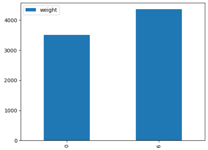
df2 = df.iloc[[0,6],3:5]
df2.plot(kind='bar')
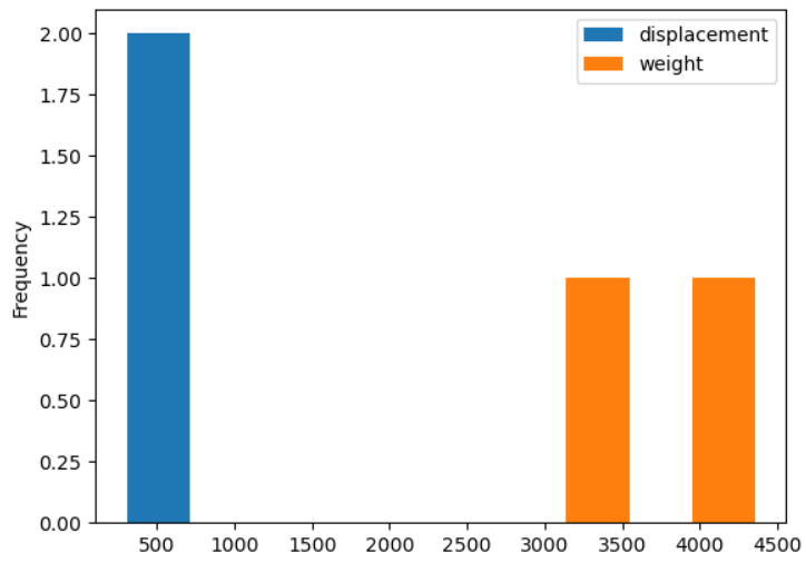
df2 = df.iloc[[0,6],2:5]
df2.plot(kind='hist')
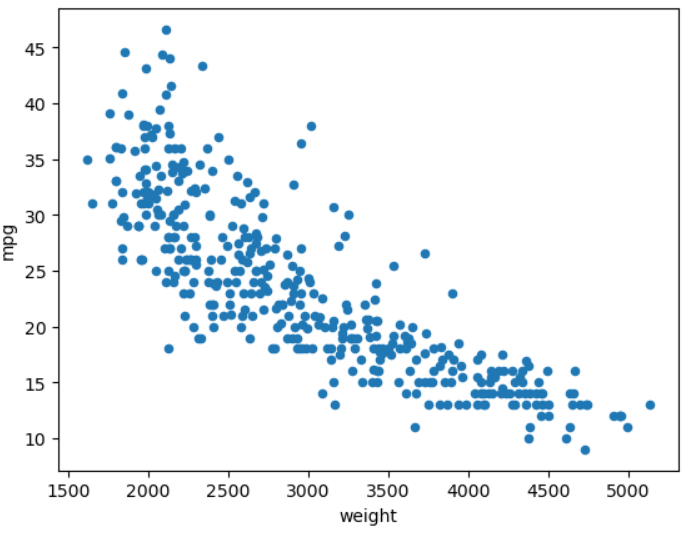
df.plot(x='weight', y='mpg', kind='scatter')
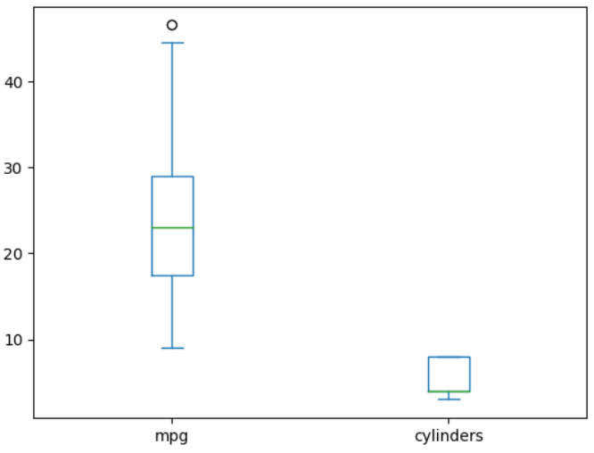
df[['mpg','cylinders']].plot(kind='box')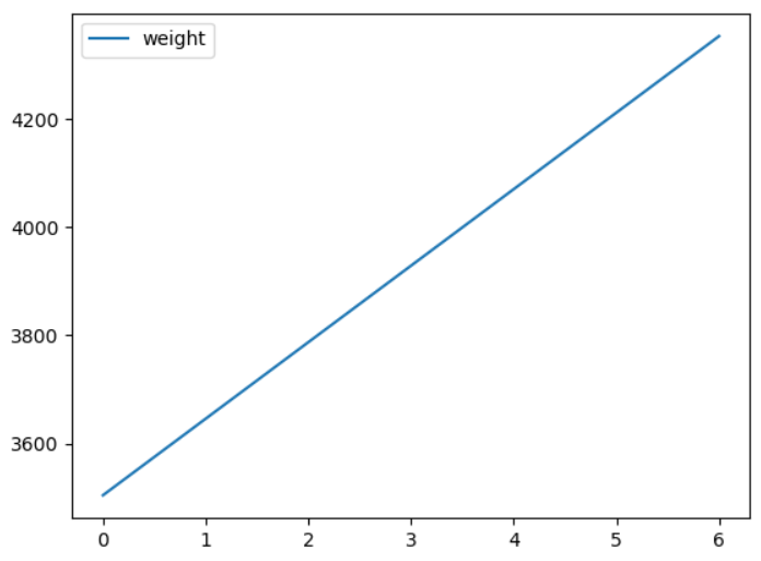
✔ 시각화 도구 - Matplotlib
# 히스토그램 (Histogram)
import matplotlib.pyplot as plt

df['mpg'].plot(kind='hist', bins=10, color='coral', figsize=(10, 5))

plt.title('Histogram')
plt.xlabel('mpg')
plt.show()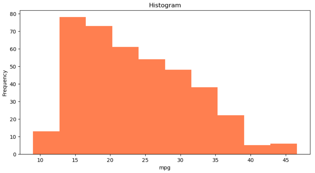
# 산점도 (Scatter)
df.plot(kind='scatter', x='weight', y='mpg', c='coral', s=10, figsize=(10,5))
plt.title('Scatter Plot - mpg vs weight')
plt.show()
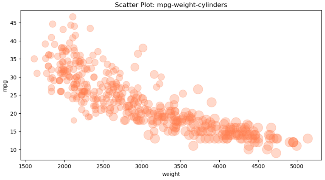
# 버블 차트 (Bubble Chart)
cylinders_size = df.cylinders/df.cylinders.max() * 300
df.plot(kind='scatter', x='weight', y='mpg', c='coral', figsize=(10,5), s=cylinders_size, alpha=0.3)
plt.title('Scatter Plot: mpg-weight-cylinders')
plt.show()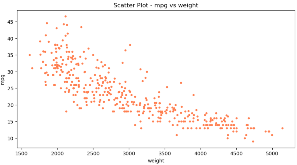
# 파이 (Pie) 차트
# -*- coding: utf-8 -*-
import pandas as pd
import matplotlib.pyplot as plt

plt.style.use('default')   # 스타일 서식 지정
df = pd.read_csv('/kaggle/input/autompg-dataset/auto-mpg.csv')
df.columns = ['mpg', 'cylinders', 'diaplacement', 'horsepower', 'weight', 'acceleration', 'model year', 'origin', 'name']

df['count'] = 1
df_origin = df.groupby('origin').sum()     # origin 열을 기준으로 그룹화, 합계 연산
print(df_origin.head())

df_origin.index  = ['USA', 'EU', 'JPN']
df_origin['count'].plot(kind='pie',
                        figsize=(7,5),
                        autopct='%1.1f%%',
                        startangle=10,     # 파이 조각을 나누는 시작점
                        colors=['chocolate','bisque','cadetblue']
                        )
plt.title('Model Origin', size=20)
plt.axis('equal')                          # 파이 차트의 비율을 같게(원에 가깝게) 조정
plt.legend(labels=df_origin.index, loc='upper right')  # 범례 표시
plt.show()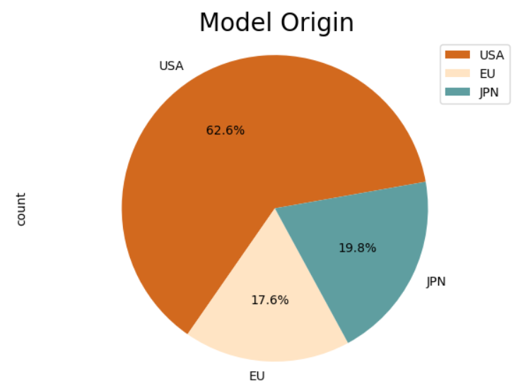
# 박스플롯 (boxplot)
fig = plt.figure(figsize=(20,10))

ax1 = fig.add_subplot(1,2,1)
ax2 = fig.add_subplot(1,2,2)

ax1.boxplot(x=[df[df['origin']==1]['mpg'],
               df[df['origin']==2]['mpg'],
               df[df['origin']==3]['mpg']],
         labels=['USA','EU','JPN'])

ax2.boxplot(x=[df[df['origin']==1]['mpg'],
               df[df['origin']==2]['mpg'],
               df[df['origin']==3]['mpg']],
         labels=['USA','EU','JPN'], vert=False)

plt.show()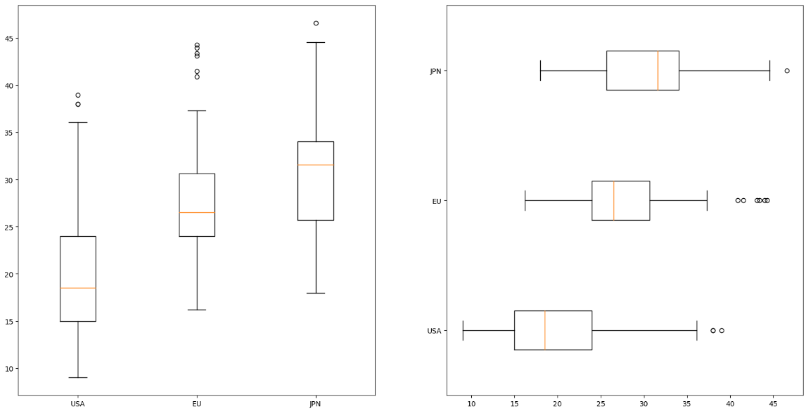
✔ 시각화 도구 - Seaborn
# titanic data 가져오기
import seaborn as sns

titanic = sns.load_dataset('titanic')
print(titanic.head())
print('\n')
print(titanic.info())

   survived  pclass     sex   age  sibsp  parch     fare embarked  class  \
0         0       3    male  22.0      1      0   7.2500        S  Third
1         1       1  female  38.0      1      0  71.2833        C  First
2         1       3  female  26.0      0      0   7.9250        S  Third
3         1       1  female  35.0      1      0  53.1000        S  First
4         0       3    male  35.0      0      0   8.0500        S  Third

     who  adult_male deck  embark_town alive  alone
0    man        True  NaN  Southampton    no  False
1  woman       False    C    Cherbourg   yes  False
2  woman       False  NaN  Southampton   yes   True
3  woman       False    C  Southampton   yes  False
4    man        True  NaN  Southampton    no   True


<class 'pandas.core.frame.DataFrame'>
RangeIndex: 891 entries, 0 to 890
Data columns (total 15 columns):
 #   Column       Non-Null Count  Dtype
---  ------       --------------  -----
 0   survived     891 non-null    int64
 1   pclass       891 non-null    int64
 2   sex          891 non-null    object
 3   age          714 non-null    float64
 4   sibsp        891 non-null    int64
 5   parch        891 non-null    int64
 6   fare         891 non-null    float64
 7   embarked     889 non-null    object
 8   class        891 non-null    category
 9   who          891 non-null    object
 10  adult_male   891 non-null    bool
 11  deck         203 non-null    category
 12  embark_town  889 non-null    object
 13  alive        891 non-null    object
 14  alone        891 non-null    bool
dtypes: bool(2), category(2), float64(2), int64(4), object(5)
memory usage: 80.7+ KB
None
✔ 회귀선이 있는 산점도
sns.set_style('darkgrid')

fig = plt.figure(figsize=(15,5))
ax1 = fig.add_subplot(1,2,1)
ax2 = fig.add_subplot(1,2,2)

# 선형회귀선 표시 (fit_reg=True)
sns.regplot(x='age', y='fare', data=titanic, ax=ax1)

# 선형회귀선 미표시 (fit_reg=False)
sns.regplot(x='age', y='fare', data=titanic, ax=ax2,
            fit_reg=False)

plt.show()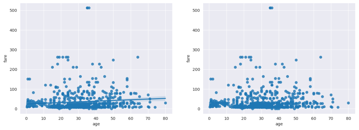
✔ 히트맵
table = titanic.pivot_table(index=['sex'], columns=['class'], aggfunc='size')

sns.heatmap(table,annot=True, fmt='d', cmap='YlGnBu', linewidth=.5, cbar=False)
plt.show()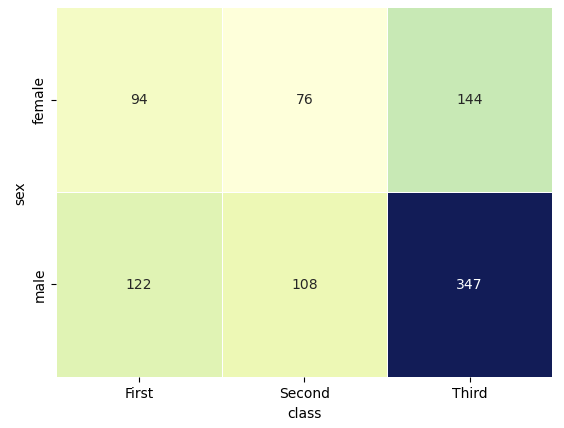
✔ 막대그래프
fig = plt.figure(figsize=(15,5))
ax1 = fig.add_subplot(1,3,1)
ax2 = fig.add_subplot(1,3,2)
ax3 = fig.add_subplot(1,3,3)

sns.barplot(x='sex', y='survived', data=titanic, ax=ax1)
sns.barplot(x='sex', y='survived', hue='class', data=titanic, ax=ax2)
sns.barplot(x='sex', y='survived', hue='class', dodge=False, data=titanic, ax=ax3)

ax1.set_title('titanic survived - sex')
ax2.set_title('titanic survived - sex/class')
ax3.set_title('titanic survived - sex/class(stacked)')

plt.show()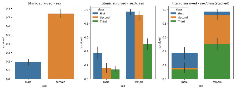
✔ 빈도그래프
fig = plt.figure(figsize=(15,5))
ax1 = fig.add_subplot(1,3,1)
ax2 = fig.add_subplot(1,3,2)
ax3 = fig.add_subplot(1,3,3)

sns.countplot(x='sex', palette='Set1', data=titanic, ax=ax1)
sns.countplot(x='sex', hue='who', palette='Set2', data=titanic, ax=ax2)
sns.countplot(x='sex', hue='who', palette='Set3', dodge=False, data=titanic, ax=ax3)

ax1.set_title('titanic survived')
ax2.set_title('titanic survived - who')
ax3.set_title('titanic survived - who(stacked)')

plt.show()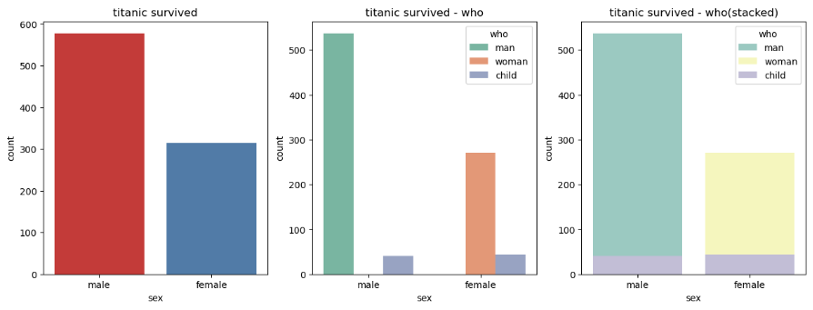
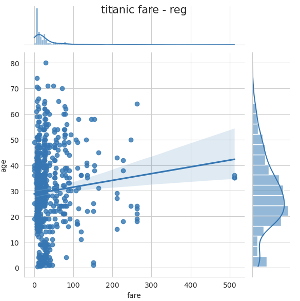
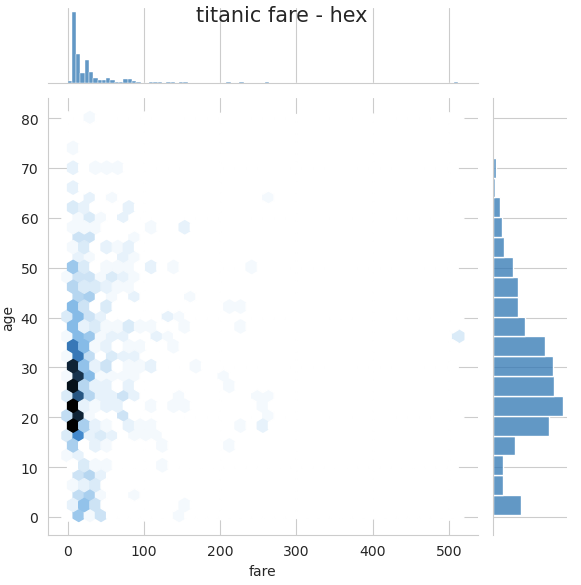
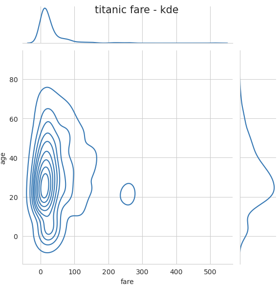
✔ 조인트 그래프
import matplotlib.pyplot as plt
import seaborn as sns

titanic = sns.load_dataset('titanic')

sns.set_style('whitegrid')

j1 = sns.jointplot(x='fare', y='age', data=titanic)
j2 = sns.jointplot(x='fare', y='age', kind='reg', data=titanic)
j3 = sns.jointplot(x='fare', y='age', kind='hex', data=titanic)
j4 = sns.jointplot(x='fare', y='age', kind='kde', data=titanic)

j1.fig.suptitle('titanic fare - scatter', size=15)
j2.fig.suptitle('titanic fare - reg', size=15)
j3.fig.suptitle('titanic fare - hex', size=15)
j4.fig.suptitle('titanic fare - kde', size=15)

plt.show()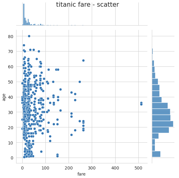
반응형
'Python' 카테고리의 다른 글
| [Python] Pandas _ Apply, Map (0) | 2023.08.24 |
|---|---|
| [Python] Pandas data 처리 (0) | 2023.05.01 |
| [Python] matplotlib, seaborn 막대그래프 그리기 / 꾸미기 (0) | 2023.04.17 |
| [Python] docstring (문서화 / 사용자 정의 함수 ) (0) | 2023.04.13 |
| [Python] Pandas Data Analysis (0) | 2023.04.13 |

